10 Essential Excel Functions for Small Business Owners (With Real Examples)

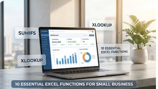
Mastering essential excel functions for small business operations is what separates a fragile workbook from an automated, reliable reporting system. Most business owners spend hours manually copying numbers, updating monthly tabs, or hunting down how to correct a #VALUE! error simply because they rely on basic arithmetic instead of dedicated formulas.

Excel contains hundreds of built-in worksheet functions, but small business owners, freelancers, and lean teams only need a core set of 10 formulas to run cash flow tracking, sales pipelines, client billing, and monthly dashboards.

The 4 Formula Categories Every Small Business Needs

To build scalable business reports, organize your formula toolkit into four distinct operational jobs:

1. Aggregation & Tracking: SUMIFS, COUNTIFS, AVERAGEIFS
2. Data Retrieval: XLOOKUP, FILTER, UNIQUE
3. Data Sanitization: TRIM, PROPER, EOMONTH
4. Logic & Governance: IFERROR, IFS

Essential Excel Functions for Small Business: Financial & Sales Aggregation

1. SUMIFS: Multi-Criteria Financial Tracking

While =SUM() adds an entire column, SUMIFS calculates totals based on one or more specific criteria—such as calculating total revenue from a specific client within a defined date range.

Syntax:

Excel

=SUMIFS(sum_range, criteria_range1, criteria1, [criteria_range2, criteria2], ...)

Practical Business Example:

Suppose you have a master sales table (tbl_Sales) with columns: Amount, Status, and Category. To sum all cleared revenue from “Consulting”:

Excel

=SUMIFS(tbl_Sales[Amount], tbl_Sales[Category], "Consulting", tbl_Sales[Status], "Paid")

Pro Tip: Always default to SUMIFS rather than legacy SUMIF. SUMIFS supports unlimited conditions and places the sum_range first, maintaining a consistent syntax structure.

2. COUNTIFS: Volume & Pipeline Auditing

COUNTIFS counts the number of rows that meet multiple conditions. It is ideal for monitoring unfulfilled orders, overdue client accounts, or monthly lead volume.

Syntax:

Excel

=COUNTIFS(criteria_range1, criteria1, [criteria_range2, criteria2], ...)

Practical Business Example:

To calculate how many invoices are currently marked "Overdue" for values exceeding $1,000:

Excel

=COUNTIFS(tbl_Invoices[Status], "Overdue", tbl_Invoices[Balance], ">1000")

3. AVERAGEIFS: Calculating Unit Economics & Average Order Value (AOV)

Tracking overall revenue is incomplete without knowing your Average Order Value (AOV) or average project size per client type. AVERAGEIFS computes the arithmetic mean for rows matching specific filters.

Syntax:

Excel

=AVERAGEIFS(average_range, criteria_range1, criteria1, [criteria_range2, criteria2], ...)

Practical Business Example:

To calculate the average transaction value for online store sales in your “Wholesale” segment:

Excel

=AVERAGEIFS(tbl_Orders[Order_Total], tbl_Orders[Channel], "Wholesale", tbl_Orders[Status], "Completed")

Data Matching & Lookup Functions

4. XLOOKUP: Dynamic Cross-Sheet Data Retrieval

XLOOKUP replaces legacy VLOOKUP and INDEX/MATCH. It searches a column for a match and returns a corresponding value from another column. It does not break when you insert new columns, searches both left and right, and handles missing data natively.

Syntax:

Excel

=XLOOKUP(lookup_value, lookup_array, return_array, [if_not_found], [match_mode])

Practical Business Example:

Match a product SKU on an invoice sheet to return the unit price from your master inventory table (tbl_Inventory):

Excel

=XLOOKUP(A2, tbl_Inventory[SKU], tbl_Inventory[UnitPrice], "SKU Not Found")

Master Inventory Table (tbl_Inventory):

SKU	Item_Description	UnitPrice
PRD-101	Web Design Package	$1,500.00
PRD-102	SEO Audit Report	$750.00

Invoice Line Calculation (Cell C2): =XLOOKUP(A2, tbl_Inventory[SKU], tbl_Inventory[UnitPrice], 0)

Result for PRD-102: $750.00

5. UNIQUE & FILTER: Automated Dynamic Lists

Instead of manually copying client names to create summary tables, modern dynamic array formulas extract clean sub-lists automatically.

A. Extracting Unique Customer or Category Lists:

Excel

=UNIQUE(tbl_Sales[Customer_Name])

Spills a deduplicated list of every client into your summary tab without manual filtering.

Read Also: What Business Data Should a Small Business Track Every Week?

B. Filtering Live Transaction Lists:

Excel

=FILTER(tbl_Invoices, tbl_Invoices[Status]="Unpaid", "No Unpaid Invoices")

Generates a live, updating table containing only unpaid accounts without manual copy-pasting.

Data Cleaning & Sanitization Functions

Raw transaction exports from Stripe, QuickBooks, Shopify, or banks are often plagued with inconsistent spacing, irregular casing, or non-standard date formats.

Raw CSV Import: ” acme corporation ” (Trailing spaces break lookups)

Cleaned via TRIM: “acme corporation”

Cleaned via PROPER: “Acme Corporation”

6. TRIM: Removing Hidden Whitespace

Invisible trailing or leading spaces inside imported data are the leading cause of #N/A errors in XLOOKUP and mismatched SUMIFS totals.

Excel

=TRIM(A2)

You May Also Like: 10 Excel Mistakes That Can Ruin Small Business Reports (And How to Fix Them)

7. PROPER & UPPER: Standardizing Text Formatting

• =PROPER(A2) capitalizes the first letter of each word (e.g., converts "john doe" to "John Doe").
• =UPPER(A2) converts text to all uppercase (e.g., standardizing state abbreviations or tax IDs like "tx" to "TX").

8. EOMONTH: Dynamic Monthly Period Calculations

To build rolling monthly financial reports, avoid hardcoding date boundaries like "2026-03-31". Use EOMONTH to automatically return the last calendar day of any month.

Syntax:

Excel

=EOMONTH(start_date, months)

Dynamic Monthly Revenue Formula:

Excel

=SUMIFS(
tbl_Ledger[Amount],
tbl_Ledger[Date], “>=” & B$1,
tbl_Ledger[Date], “<=” & EOMONTH(B$1, 0)
)

Where cell B$1 holds the first day of the reporting month (e.g., 2026-03-01).

Logic & Error-Proofing Functions

9. IFERROR: Preventing Broken Dashboard Visuals

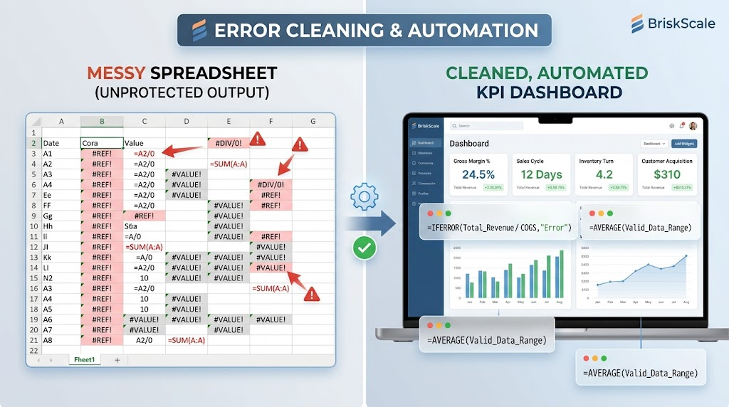
When formulas attempt to divide by zero (e.g., calculating conversion rate when traffic is zero) or fail a lookup, Excel displays #DIV/0! or #N/A. IFERROR catches these errors and replaces them with a clean default value.

Syntax:

Excel

=IFERROR(value, value_if_error)

Practical Business Example:

Excel

=IFERROR(C2 / B2, 0)

Calculates conversion rate (Sales / Leads); returns 0 instead of #DIV/0! if Leads are zero.

10. IFS: Handling Multi-Condition Business Logic

When assigning customer tiers, commission rates, or payment priority, avoid deeply nested =IF(IF(IF())) chains. IFS tests multiple conditions in a single readable line.

Syntax:

Excel

=IFS(condition1, value1, [condition2, value2], ...)

Practical Business Example (Sales Commission Tiers):

Excel

=IFS(
    D2 >= 50000, 0.15,
    D2 >= 20000, 0.10,
    D2 >= 5000, 0.05,
    TRUE, 0.00
)

Evaluates sales volume in cell D2 and returns the matching commission percentage. The final TRUE, 0.00 serves as the fallback catch-all.

Small Business Excel Functions Quick-Reference Cheat Sheet

Function	Primary Small Business Use Case	Example Formula
SUMIFS	Multi-condition revenue and expense aggregation	=SUMIFS(tbl_Exp[Amount], tbl_Exp[Category], "Software")
COUNTIFS	Tracking volume of open orders or late payments	=COUNTIFS(tbl_Inv[Status], "Late", tbl_Inv[Days], ">30")
AVERAGEIFS	Measuring Average Order Value (AOV) by channel	=AVERAGEIFS(tbl_Sales[Amount], tbl_Sales[Type], "Retail")
XLOOKUP	Matching item prices, client emails, or vendor IDs	=XLOOKUP(A2, tbl_Items[SKU], tbl_Items[Price], 0)
UNIQUE	Generating dynamic lists of active clients or SKUs	=UNIQUE(tbl_Orders[Client_Name])
FILTER	Spilling a live sub-table of overdue invoices	=FILTER(tbl_Invoices, tbl_Invoices[Status]="Unpaid")
TRIM	Cleaning whitespace out of imported CSV files	=TRIM(RawData!A2)
PROPER	Standardizing client names and vendor formatting	=PROPER(RawData!B2)
EOMONTH	Finding the dynamic end-date of any financial period	=EOMONTH(B1, 0)
IFERROR	Masking ugly calculation errors on public dashboards	=IFERROR(A2/B2, 0)

3 Best Practices for Writing Durable Business Formulas

1. Use Formal Excel Tables (Ctrl + T): Always convert raw ranges into named Excel Tables. This allows formulas to use structured references (tbl_Sales[Amount]) that automatically expand when new data is entered.
2. Never Hardcode Numbers Inside Formulas: Never write =SUM(A2:A50) * 1.0825. Place the tax rate (8.25%) into a dedicated parameter cell (e.g., cell Settings!B2) and reference that cell directly.
3. Keep Raw Data and Formula Outputs on Separate Sheets: Maintain a strict separation between where transactions are entered (Input tabs) and where formulas generate executive summaries (Output tabs).

Read Also: 10 Business Processes Small Businesses Should Stop Managing Manually

Frequently Asked Questions